10 mins to GFQL: ICIJ FinCEN Files Visualization
This document will serve as an end-to-end demonstration of using Graphistry's GFQL to extract information out of a complex real-world dataset. For this purpose, we will use a dataset made available by the International Consortium of Investigative Journalists (ICIJ) as part of their reporting of leaked documents from the U.S. Department of Treasury’s Financial Crimes Enforcement Network, which include suspicious activity reports filed by U.S. banks acting as beneficiary or orginating banks in domestic transactions or as correspondent or intermediary banks in international transactions. More information about the dataset can be found at the ICIJ.
Data downloaded from the ICIJ will be loaded into Graphistry, suspected suspicious transactions to alleged “high risk” jurisdictions in the Caribbean will be analyzed, and a suspicious transaction linked to Oleg Deripaska; one of the confidential clients highlighted by the ICIJ will be isolated.
This demonstration will be done using Graphistry's Python library, however REST endpoints which permit access to GFQL querying of uploaded datasets are available.
To run the code in this demonstration, please login using your Graphistry account in order to obtain access to server-side visualization endpoints needed to render extracted subgraphs.
import graphistry

graphistry.register(api=3, protocol="https", server="hub.graphistry.com",
                    username="...", password="...")
First, download the dataset from the ICIJ and read the download_transactions_map.csv file containing bank-to-bank transaction data into a dataframe. This data is used as an edgelist to initialize a Graphistry graph, with the originator_bank_id identifying the edge source and the beneficiary_bank_id identifying the edge destination. The edge source and destination IDs are used to synthesize the graph nodes.
Note that while we could greatly benefit from doing some data preprocessing, we have deliberately chosen not to in order to highlight the flexibility of using GFQL to work around the unprocessed data and simplify the demonstration.
import requests
import zipfile
import pandas as pd

# download data
resp = requests.get("https://media.icij.org/uploads/2020/09/download_data_fincen_files.zip")
with open("download_data_fincen_files.zip", "wb") as f:
    f.write(resp.content)
with zipfile.ZipFile("download_data_fincen_files.zip","r") as zip_ref:
    zip_ref.extract("download_transactions_map.csv")

# read csv into pandas dataframe and change type of time columns in data to datetime
df_e = pd.read_csv("download_transactions_map.csv")
df_e["begin_date"] = pd.to_datetime(df_e["begin_date"])
df_e["end_date"] = pd.to_datetime(df_e["end_date"])

# create graph
g = graphistry.edges(df_e, "originator_bank_id", "beneficiary_bank_id").materialize_nodes()

# rename id col in nodes to nodeId
df_n = g._nodes.rename(columns={'id': 'nodeId'})
g = g.nodes(df_n, 'nodeId')
Node-list sample
| nodeId |
|---|
| cimb-bank-berhad |
| barclays-bank-plc-ho-uk |
| natwest-offshore |
| ... |
Edge-list sample
| id | icij_sar_id | filer_org_name_id | filer_org_name | begin_date | end_date | originator_bank_id | originator_bank | originator_bank_country | originator_iso | beneficiary_bank_id | beneficiary_bank | beneficiary_bank_country | beneficiary_iso | number_transactions | amount_transactions |
|---|---|---|---|---|---|---|---|---|---|---|---|---|---|---|---|
| 223254 | 3297 | the-bank-of-new-york-mellon-corp | The Bank of New York Mellon Corp. | 2015-03-25 | 2015-09-25 | cimb-bank-berhad | CIMB Bank Berhad | Singapore | SGP | barclays-bank-plc-london-england-gbr | Barclays Bank Plc | United Kingdom | GBR | 68.0 | 56898523.47 |
| 223255 | 3297 | the-bank-of-new-york-mellon-corp | The Bank of New York Mellon Corp. | 2015-03-30 | 2015-09-25 | cimb-bank-berhad | CIMB Bank Berhad | Singapore | SGP | barclays-bank-plc-london-england-gbr | Barclays Bank Plc | United Kingdom | GBR | 118.0 | 56898523.47 |
| 223258 | 2924 | the-bank-of-new-york-mellon-corp | The Bank of New York Mellon Corp. | 2012-07-05 | 2012-07-05 | barclays-bank-plc-ho-uk | Barclays Bank Plc Ho UK | United Kingdom | GBR | skandinaviska-enskilda-banken-stockholm-sweden-swe | Skandinaviska Enskilda Banken | Sweden | SWE | 56898523.47 | |
| ... | ... | ... | ... | ... | ... | ... | ... | ... | ... | ... | ... | ... | ... | ... | ... |
The graph visualizations will be rendered as follows.
Node colours will be assigned on a per-graph basis. Edge colours will encode the transaction amount where there is more than 1 edge present, and will vary from "purple" to "blue" to "green" to "yellow" according to the "Viridis" palette as the transaction amount encoded in an edge increases. A nonlinear_palette_generator function will be used to hand tune non-linearity values for each graph to optimize the colour mapping for the exponentially distributed transaction amount data.
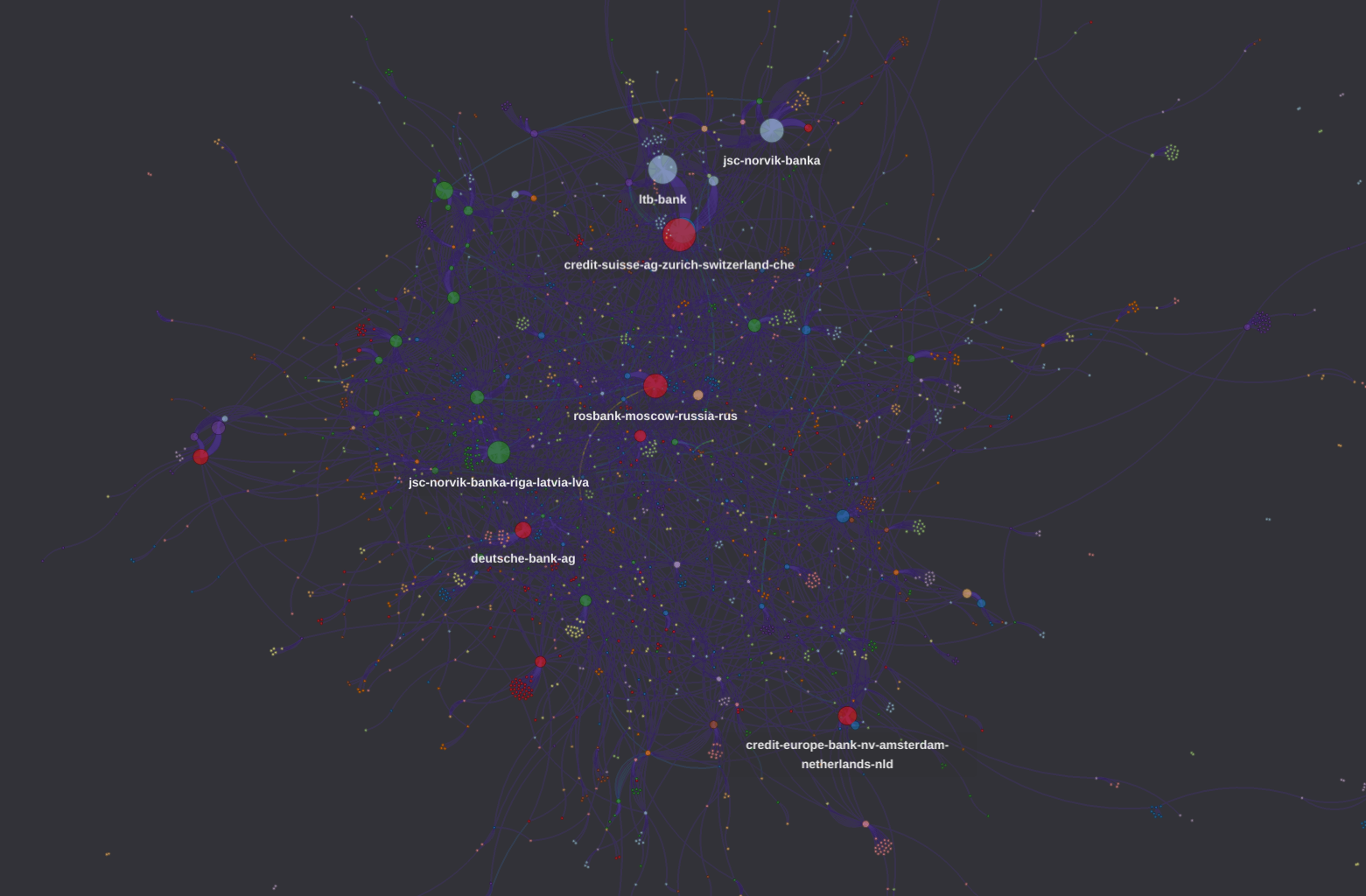
Next, lets visualize the entire graph.
# declare helper functions and variables
def nonlinear_palette_generator(v, linear_palette):
    out = []
    num_palette = len(linear_palette)
    num_palette_repetitions = [round(n**v) + 1 for n in range(num_palette)]
    if v < 1:
        num_palette_repetitions.reverse()
    for i, color in enumerate(linear_palette):
        out = out + [color for _ in range(num_palette_repetitions[i])]
    return out

palette = ["#46327e", "#365c8d", "#277f8e", "#1fa187", "#4ac16d", "#a0da39", "#fde725"]

# render graph of entire dataset
g_out = g.bind(edge_label="amount_transactions")
g_out = g_out.encode_edge_color("amount_transactions",
                                nonlinear_palette_generator(1.2, palette),
                                as_continuous=True)
g_out = g_out.settings(
    height=800,
    url_params={
        "pointOpacity": 0.6 if len(g_out._nodes) > 1500 else 0.9,
        "edgeOpacity": 0.3 if len(g_out._edges) > 1500 else 0.9,
        "play": 2000})
g_out.plot()
Caribbean havens subgraph
The ICIJ mentions the importance of the world's top offshore financial havens in the data. Therefore, lets look at a subgraph containing transactions to and from a handful of the most well known Caribbean financial havens and observe where transactions are happening.
We have created a list of chain operations consisting of two members:
e_forwardoperation matches for all transactions where the originator country is in that list. The edge operation specifies forward to enable the next operation.noperation matches for all nodes but since it is followed by thee_forwardoperation which filters for transactions originating from countries in the list, we can assume that all nodes such edges originating from must be Caribbean. These nodes are tagged with the nameis_carib_bank_originto encode colours during visualization.
from graphistry import n, e_forward, is_in

carib_havens = [
    "Cayman Islands",
    "Bermuda",
    "Virgin Islands British",
    "British Virgin Islands",
    "Bahamas",
    "Panama",
    "Barbados",
]

# render transactions out of the Caribbean
chain_operations = graphistry.Chain([
    n(name="is_carib_bank_origin"),
    e_forward(hops=1, edge_match={"originator_bank_country": is_in(options=carib_havens)}),
])
g_carib_out = g.chain(chain_operations)

g_carib_out = g_carib_out.bind(edge_label="amount_transactions")
g_carib_out = g_carib_out.encode_edge_color("amount_transactions",
                                            nonlinear_palette_generator(1.4, palette),
                                            as_continuous=True)
g_carib_out = g_carib_out.encode_point_color("is_carib_bank_origin",
                                              as_categorical=True,
                                              categorical_mapping={True: "red", False: "blue"})
g_carib_out = g_carib_out.settings(
            height=800,
            url_params={
                "pointOpacity": 0.6 if len(g_carib_out._nodes) > 1500 else 0.9,
                "edgeOpacity": 0.3 if len(g_carib_out._edges) > 1500 else 0.9,
                "strongGravity": True,
                "play": 2000})
g_carib_out.plot()

# render transactions into the Caribbean
from graphistry import n, e_forward, is_in

chain_operations = graphistry.Chain([e_forward(hops=1,
                                    edge_match={"beneficiary_bank_country": is_in(options=carib_havens)}),
                                    n(name="is_carib_bank_destination")])
g_carib_in = g.chain(chain_operations)

g_carib_in = g_carib_in.bind(edge_label="amount_transactions")
g_carib_in = g_carib_in.encode_edge_color("amount_transactions",
                                          nonlinear_palette_generator(1.4, palette),
                                          as_continuous=True)
g_carib_in = g_carib_in.encode_point_color("is_carib_bank_destination",
                                            as_categorical=True,
                                            categorical_mapping={True: "red", False: "blue"})
g_carib_in = g_carib_in.settings(
            height=800,
            url_params={
                "pointOpacity": 0.6 if len(g_carib_in._nodes) > 1500 else 0.9,
                "edgeOpacity": 0.3 if len(g_carib_in._edges) > 1500 else 0.9,
                "strongGravity": True,
                "play": 2000})
g_carib_in.plot()
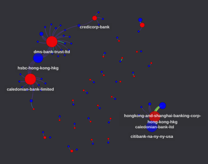
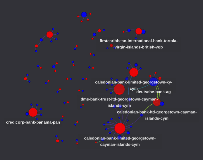
There are some patterns present in the two graphs. Despite how there were 6 countries in the list, the banks with the greatest number of suspicious transactions are in the Cayman Islands. There are also not insignificant transactions from the Virgin Islands too.
The country recieving the most funds from the listed Caribbean countries is Hong Kong, with most of it heading to HSBC HK from Caledonian Bank of the Cayman Islands.
The country sending the most funds to the listed Caribbean countries is the UK to the Caledonian Bank of the Cayman islands, primarily due to 3 transactions sent within days of each other totalling roughly 600 million dollars.
Single transaction subgraph
Next lets try to find a suspicious transaction the ICIJ linked to Oleg Deripaska; a Russian oligarch. According to the ICIJ:
- On Aug. 15, 2013, Mallow Capital Corp., in the British Virgin Islands, sent $15.9 million from its account at Expobank in Latvia
- The funds were sent to Deutsche Bank Trust Company Americas in New York.
- Deutsche Bank U.S. then sent the funds to the Bank of New York Mellon, which later flagged the transaction as suspicious.
- The funds were then credited to Mallow Capital’s account at Bank Soyuz in Russia. The transaction was labeled a “funds transfer”.
Lets try to cast a wider net at first rather than dive straight in. Because of the dataset structure, we can ignore the American corresponding and intermediary banks in the fact list. Lets extract a subgraph containing all transactions from Latvian banks to Russian Banks.
We have created a list of chain operations consisting of two members:
e_forwardoperation matches for all transactions where the benefiary country isRussiaand the originator country isLatvia. The edge operation specifies forward in order to enable the next operation.e_forwardoperation matches for all nodes but since it is preceded by thee_forwardoperation which filters for transactions heading to Russia, we can assume that all nodes such edges are going to must be Russian. These nodes are tagged with the nameis_rus_beneficiaryto encode colours during visualization.
from graphistry import n, e_forward, contains

# render transactions from Latvia into Russia
chain_operations = graphistry.Chain([
    e_forward(hops=1,
              edge_match={"originator_bank_country": "Latvia", "beneficiary_bank_country": "Russia"}),
    n({"nodeId": contains(pat="")}, name="is_rus_beneficiary"),
])
g_lva_rus = g.chain(chain_operations)

g_lva_rus = g_lva_rus.bind(edge_label="amount_transactions")
g_lva_rus = g_lva_rus.encode_edge_color("amount_transactions",
                                        nonlinear_palette_generator(1.4, palette), as_continuous=True)
g_lva_rus = g_lva_rus.encode_point_color("is_rus_beneficiary",
                                          as_categorical=True,
                                          categorical_mapping={True: "red", False: "blue"})
g_lva_rus = g_lva_rus.settings(
            height=800,
            url_params={
                "pointOpacity": 0.6 if len(g_lva_rus._nodes) > 1500 else 0.9,
                "edgeOpacity": 0.3 if len(g_lva_rus._edges) > 1500 else 0.9,
                "strongGravity": True,
                "play": 2000})
g_lva_rus.plot()
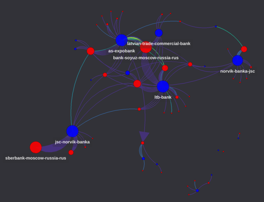
The banks mentioned in the fact list are quite prominent in the subgraph; the Latvian bank with the id as-expobank and a Russian bank with the id bank-soyuz-moscow-russia-rus are the most active pair in the subgraph by dollar amount transacted. The transaction of interest can be found by looking through the 9 transactions between the two banks in the fact list, or GFQL can be used to cut things down even further.
We have created a list of chain operations consisting of three members:
e_forwardoperation matches all transactions where the benefiary country isRussia, the originator country isLatvia, and the transaction amount is between 15.8 million and 16 million. The edge operation specifies forward in order to enable the next operation.- First
noperation matches for all nodes where thenodeIdcontains the substringexpo, but since it is followed by thee_forwardoperation which filters for transactions coming from Latvia between the transaction amount range15800000and16000000, it will only match nodes connected to an edge with those properties. - Second
noperation matches for all nodes where thenodeIdcontains the substringsoyuz, but since it is preceded by thee_forwardoperation which filters for transactions going to Russia between the transaction amount range15800000and16000000, it will only match nodes connected to an edge with those properties. These nodes are tagged with the nameis_soyuzto encode colours during visualization.
from graphistry import n, e_forward, contains, between

# render transaction
chain_operations = graphistry.Chain([
    n({"nodeId": contains(pat="expo")}),
    e_forward(hops=1, edge_match={
        "originator_bank_country": "Latvia",
        "beneficiary_bank_country": "Russia",
        "amount_transactions": between(15800000, 16000000)}),
    n({"nodeId": contains(pat="soyuz")}, name="is_soyuz")])
g_od = g.chain(chain_operations)

g_od = g_od.bind(edge_label="amount_transactions")
g_od = g_od.encode_point_color("is_soyuz", as_categorical=True, categorical_mapping={True: "red", False: "blue"})
g_od = g_od.settings(
            height=800,
            url_params={
                "pointOpacity": 0.3 if len(g_od._nodes) > 1500 else 0.9,
                "edgeOpacity": 0.2 if len(g_od._edges) > 1500 else 0.9,
                "strongGravity": True,
                "play": 2000})
g_od.plot()
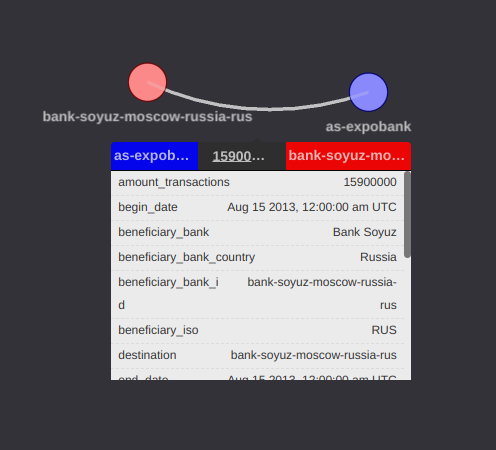
The facts indicate that we should expect only one transaction and that is exactly what we get. All the other properties match up as well; the transaction was started Aug 15 2013 and the filing US bank is the Bank of New York Mellon. This is the transaction found by the ICIJ.
In closing
This document is only intended to provide a quick introduction to how exploring data using GFQL can be accomplished, from data ingestion to formulating GFQL queries to some surface level analysis. To learn more about GFQL, please view the API documents for either Python GFQL usage (as demonstrated here), or REST endpoint GFQL usage. A document performing a deep dive into how GFQL chain works and how it can be used is available.
Finally, the Python code above is available as a notebook.